S4 generic for previewing Giotto's image and subcellular objects.
Usage
# S4 method for class 'giottoImage,missing'
plot(x, y, ...)

# S4 method for class 'giottoLargeImage,missing'
plot(
  x,
  y,
  col,
  mar,
  ext = NULL,
  xmin = NULL,
  xmax = NULL,
  ymin = NULL,
  ymax = NULL,
  legend = NULL,
  asRGB = FALSE,
  smooth = TRUE,
  axes = !add,
  plg = list(),
  maxcell = 5e+05,
  max_intensity = NULL,
  range = NULL,
  fill_range = FALSE,
  levels = NULL,
  all_levels = FALSE,
  breaks = NULL,
  breakby = "eqint",
  fun = NULL,
  colNA = NULL,
  alpha = NULL,
  sort = FALSE,
  reverse = FALSE,
  grid = FALSE,
  zebra = FALSE,
  reset = FALSE,
  add = FALSE,
  buffer = FALSE,
  background = NULL,
  box = axes,
  clip = TRUE,
  ...
)

# S4 method for class 'giottoAffineImage,missing'
plot(x, y, ...)

# S4 method for class 'giottoPolygon,missing'
plot(
  x,
  point_size = 0.6,
  type = c("poly", "centroid"),
  max_poly = getOption("giotto.plot_max_poly", 1e+06),
  ...
)

# S4 method for class 'giottoPoints,missing'
plot(
  x,
  point_size = 0,
  feats = NULL,
  raster = TRUE,
  raster_size = 600,
  count = TRUE,
  sigma = NULL,
  ...
)

# S4 method for class 'spatLocsObj,missing'
plot(x, y, ...)

# S4 method for class 'dimObj,missing'
plot(x, dims = c(1, 2), ...)

# S4 method for class 'spatialNetworkObj,missing'
plot(x, y, ...)

# S4 method for class 'affine2d,missing'
plot(x, y, ...)
Arguments
- x
giotto image, giottoPolygon, or giottoPoints object
- y
Not used.
- ...
additional parameters to pass
- col
character. Colors. The default is grDevices::grey.colors(n = 256, start = 0, end = 1, gamma = 1)
- mar
numeric vector of length 4 to set the margins of the plot (to make space for the legend). The default is (3, 5, 1.5, 1)
- ext
object that works with
ext(). Set the spatial extent of the plot.- xmin, xmax, ymin, ymax
(optional)
numeric. xy minmax ranges to use when plotting. Ifextis also provided, these are applied afterwards.- legend
logical or character. If not
FALSEa legend is drawn. The character value can be used to indicate where the legend is to be drawn. For example "topright" or "bottomleft". Useplgfor more refined placement. Not supported for continuous legends (the default for raster data)- asRGB
(optional) logical. Force RGB plotting if not automatically detected
- smooth
logical. If
TRUEthe cell values are smoothed (only if a continuous legend is used)- axes
logical. Draw axes?
- plg
list with parameters for drawing the legend. See the arguments for
legend.A legend can be placed by specifying arguments
xandy. For a continuous legendycan have two values.xcan also be a SpatExtent. Furthermore,xcan be a keyword such "topleft" and "bottomright" to place the legend at these locations inside the map rectangle. For a continuous legend, only the placement keywords "left", "right", "top", "bottom", "topright", "bottomright" are recognized; and when using these keywords, the legend is placed outside of the map rectangle. The placement of the legend can be altered with argumentnudgethat moves the location in the directions specified with one value (x direction) or two values (x, y). For a continuous legend it can also have four values (xmin, xmax, ymin, ymax). When supplying coordinates, usehoriz=TRUEto get a horizontal legend.Additional parameters for continuous legends include:
digitsinteger. The number of digits to print after the decimal pointsizeto change the height and/or width; the defaults arec(1,1)atto set the location of the tickmarksformatas informatCto format the numbers. For example, you can useformat="g"for scientific notation. The default is"f"tickOne of these partially matched values: "through", "in", "middle", "out", or "none", to choose a tickmark placement/length that is different from the default "throughout".tick.lengthto change the tickmark length (default = 1). Only relevant whentickis "throughout" or "out".tick.col,tick.box.colandtick.lwdto change the appearance of the tickmarkstitleadd a legend titletitle.srtto rotate the legend titletitle.xandtitle.yto place the legend title at specific coordinatesbgbackground color behind the legend (e.g."white") for visibility when drawn on top of a map
- maxcell
positive integer. Maximum number of cells to use for the plot
- max_intensity
(optional) value to treat as maximum intensity in color scale. Overridden by
rangeparam- range
numeric. minimum and maximum values to be used for the continuous legend. You can use
NAfor one of these to only set the minimum or maximum value- fill_range
logical. If
TRUE, values outside ofrangeget the colors of the extreme values; otherwise they get colored asNA- levels
character. labels for the legend when
type="classes"- all_levels
logical. If
TRUE, the legend shows all levels of a categorical raster, even if they are not present in the data- breaks
numeric. Either a single number to indicate the number of breaks desired, or the actual breaks. When providing this argument, the default legend becomes "interval"
- breakby
character or function. Either "eqint" for equal interval breaks, "cases" for equal quantile breaks. If a function is supplied, it should take a single argument (a vector of values) and create groups
- fun
function to be called after plotting each SpatRaster layer to add something to each map (such as text, legend, lines). For example, with SpatVector
v, you could dofun=function() lines(v). The function may have one argument, representing the layer that is plotted (1 to the number of layers)- colNA
character. color for the NA values
- alpha
Either a single numeric between 0 and 1 to set the transparency for all colors (0 is transparent, 1 is opaque) or a SpatRaster with values between 0 and 1 to set the transparency by cell. To set the transparency for a given color, set it to the colors directly
- sort
logical. If
TRUElegends with categorical values are sorted. Ifxis aSpatVectoryou can also supply a vector of the unique values, in the order in which you want them to appear in the legend- reverse
logical. If
TRUE, the legend order is reversed- grid
logical. If
TRUEgrid lines are drawn. Their properties such as type and color can be set with thepaxargument. The grid is drawn first such that it is covered byx. Seeadd_gridto add grid lines on top of the map- zebra
logical. If
TRUEa "zebra-box" is added to the axes (ignored whenadd=TRUE). The width of the zebra-box can be set with additional argumentzebra.cex. The colors can be changed with additional argumentzebra.col- reset
logical. If
TRUEthe margins (see argumentmar) are reset to what they were before calling plot; doing so may affect the display of additional objects that are added to the map (e.g. withlines)- add
logical. If
TRUEadd the object to the current plot- buffer
logical. If
TRUEthe plotting area is made slightly larger than the extent ofx- background
background color. Default is no color (white)
- box
logical. Should a box be drawn around the map?
- clip
logical. Should the axes be clipped to the extent of
x?- point_size
size of points when plotting giottoPoints
- type
what to plot: either 'poly' (default) or polygon 'centroid'
- max_poly
numeric. If
typeis not specified, maximum number of polygons to plot before automatically switching to centroids plotting. Default is 1e4. This value is settable using options("giotto.plot_max_poly")- feats
specific features to plot within giottoPoints object (defaults to NULL, meaning all available features)
- raster
default = TRUE, whether to plot points as rasterized plot with size based on
raster_sizeparam. See details. WhenFALSE, plots viaterra::plot()- raster_size
Default is 600. Only used when
rasteris TRUE- count
logical. Show point density usingcountstatistic per rasterized cell. (Default = TRUE) This param affectscolparam defaults. When TRUE,colisgrDevices::hcl.colors(256). WhenFALSE, "black" and "white" are used.- sigma
numeric(default = NULL). Amount of smoothing whencount = TRUE. SetNULLfor no smoothing. Larger values can take a while.- dims
dimensions to plot
Details
[giottoPoints raster plotting]
Fast plotting of points information by rasterizing the information using
terra::rasterize(). For terra SpatVectors, this is faster than
scattermore plotting. When plotting as a raster, col colors map on
whole image level, as opposed to mapping to individual points, as it does
when raster = FALSE
Allows the following additional params when
plotting with no specific feats input:
force_size logical.
raster_sizeparam caps at 1:1 with the spatial extent, but also with a minimum resulting px dim of 100. To ignore these constraints, setforce_size = FALSEbackground (optional) background color. Usually not used when a
colcolor mapping is sufficient.
Note that col param and other base::plot() graphical params are available
through ...
Functions
plot(x = giottoImage, y = missing): Plot magick-based giottoImage object. ... param passes to.plot_giottoimage_mgplot(x = giottoLargeImage, y = missing): Plot terra-based giottoLargeImage object. ... param passes toterra::plot()plot(x = giottoPolygon, y = missing): Plot terra-based giottoPolygon object. ... param passes toplotplot(x = giottoPoints, y = missing): terra-based giottoPoint object. ... param passes toplotplot(x = spatLocsObj, y = missing): Plot a spatLocsObjplot(x = dimObj, y = missing): Plot a dimObjplot(x = spatialNetworkObj, y = missing): Plot a spatialNetworkObjplot(x = affine2d, y = missing): Plot a affine2d. blue is start, red is end
Examples
######### giottoLargeImage plotting #########
if (FALSE) { # \dontrun{
gimg <- GiottoData::loadSubObjectMini("giottoLargeImage")
gimg <- GiottoClass:::.update_giotto_image(gimg) # only needed if out of date
plot(gimg)
plot(gimg, col = grDevices::hcl.colors(256))
plot(gimg, max_intensity = 100)
} # }
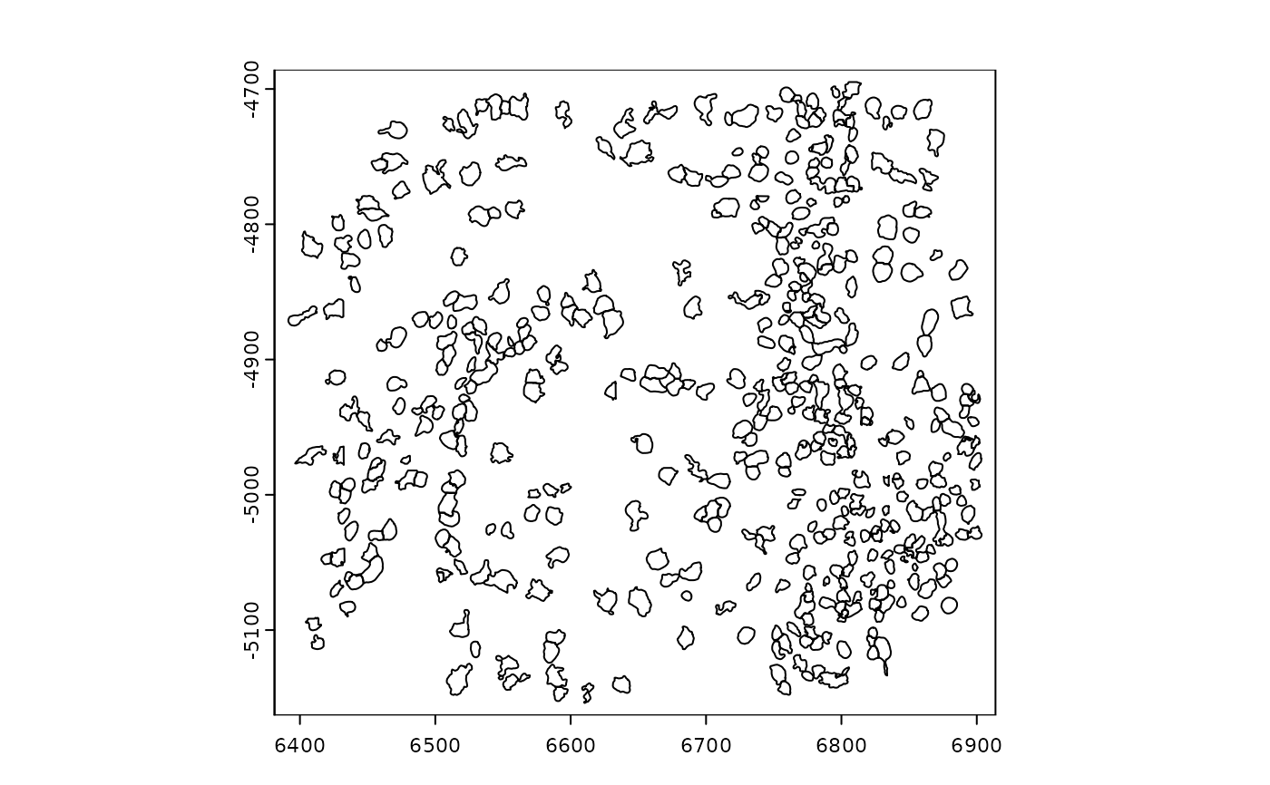
######### giottoPolygon plotting #########
gpoly <- GiottoData::loadSubObjectMini("giottoPolygon")
plot(gpoly)
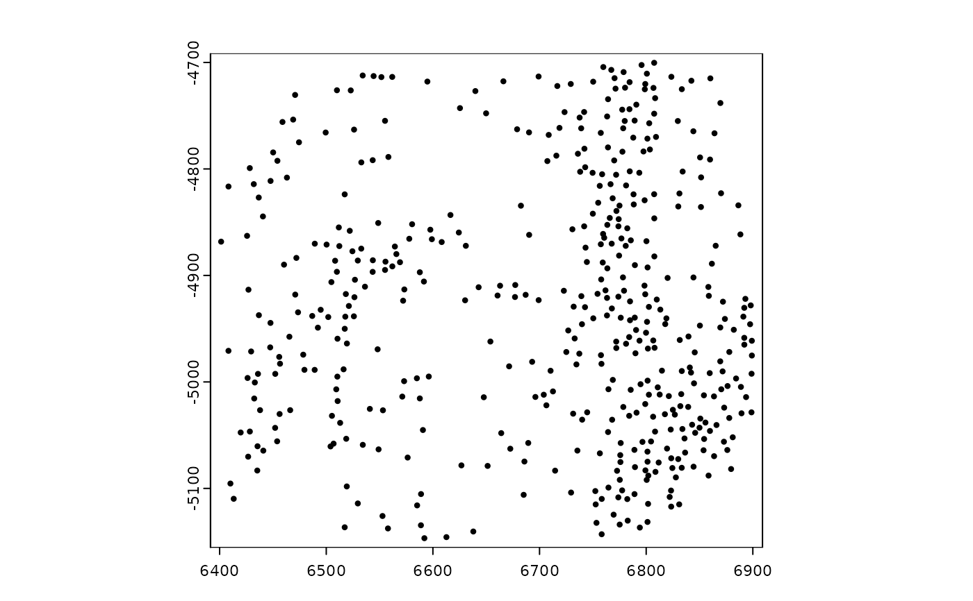
 plot(gpoly, type = "centroid")
 ######### giottoPoints plotting #########
gpoints <- GiottoData::loadSubObjectMini("giottoPoints")
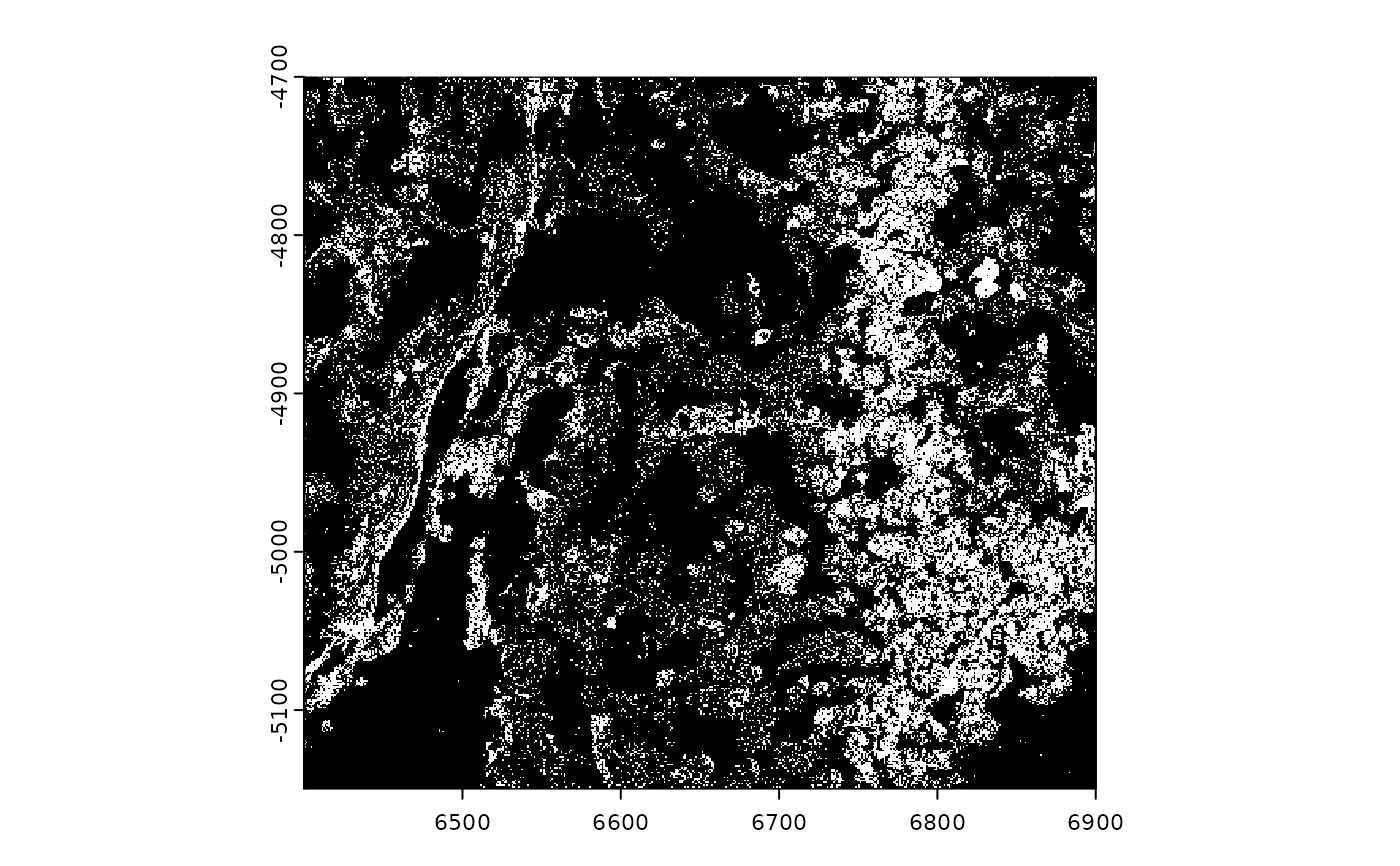
# ----- rasterized plotting ----- #
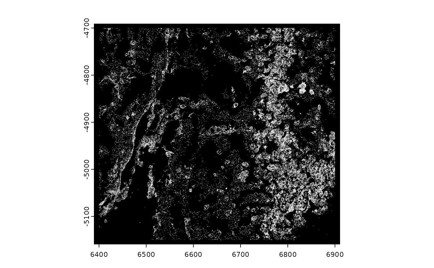
# plot points binary
plot(gpoints, count = FALSE)
######### giottoPoints plotting #########
gpoints <- GiottoData::loadSubObjectMini("giottoPoints")
# ----- rasterized plotting ----- #
# plot points binary
plot(gpoints, count = FALSE)
 # plotting all features maps colors on an image level
plot(gpoints, col = grDevices::hcl.colors(n = 256)) # only 2 colors are used
# plotting all features maps colors on an image level
plot(gpoints, col = grDevices::hcl.colors(n = 256)) # only 2 colors are used
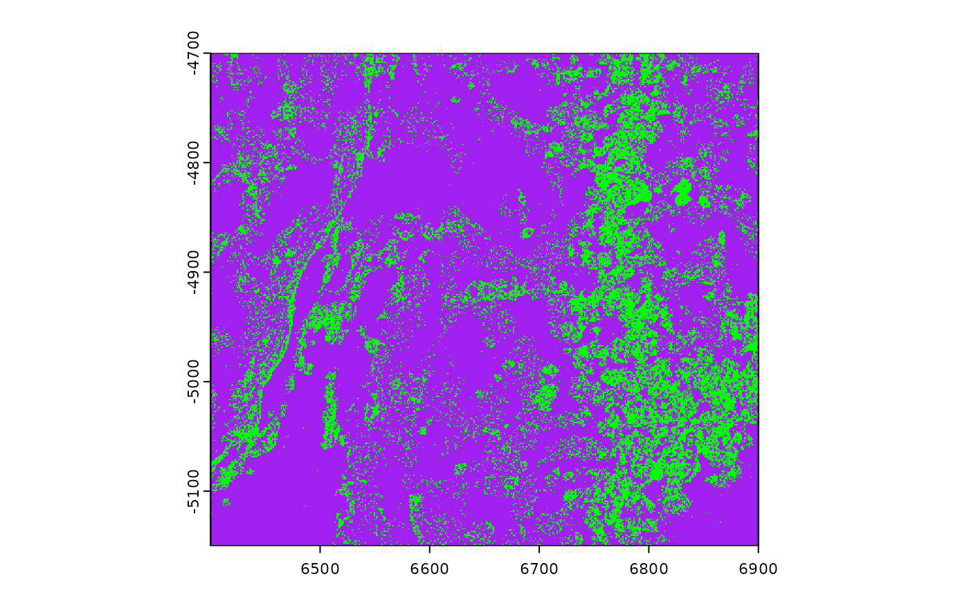
 plot(gpoints, col = "green", background = "purple")
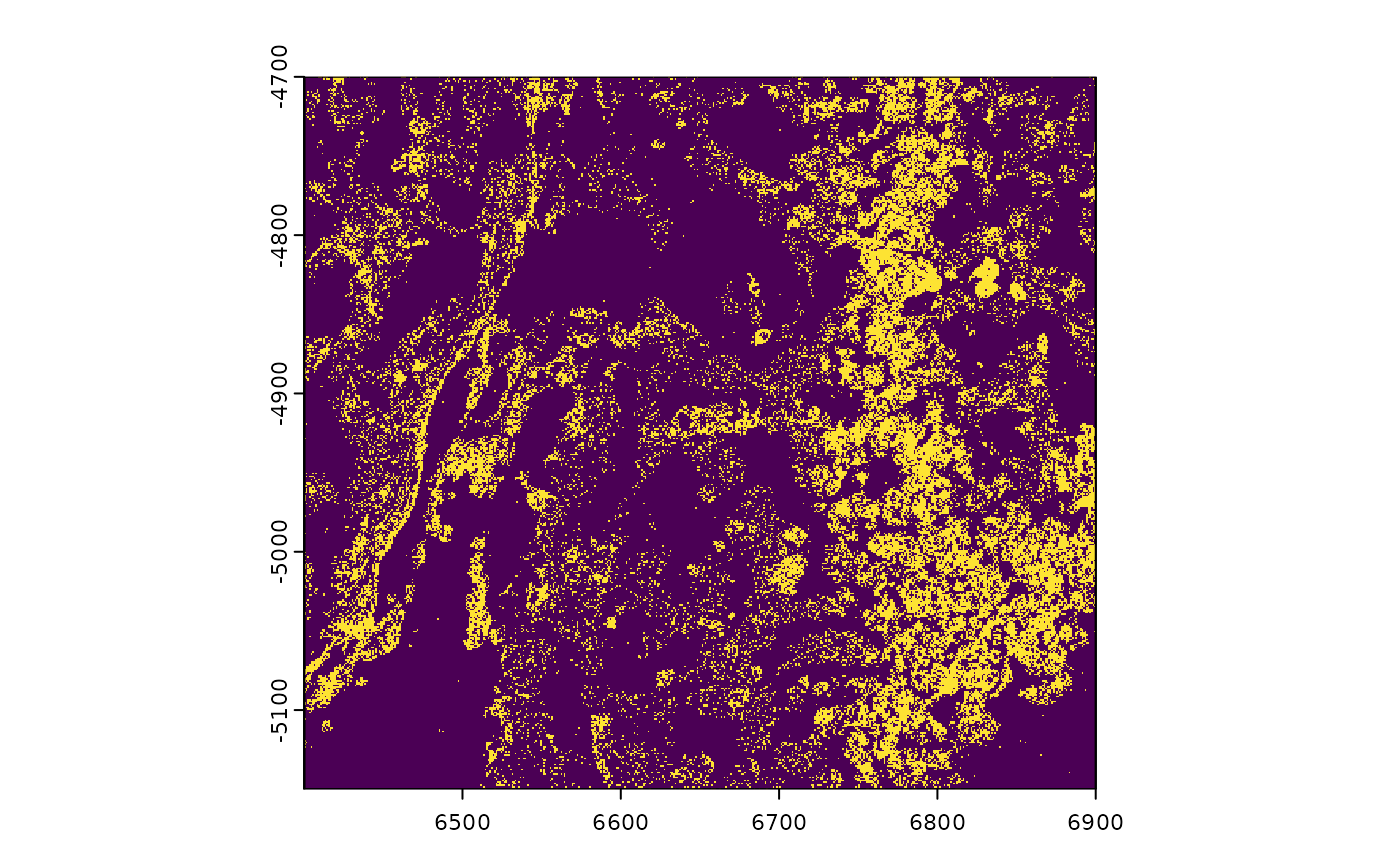
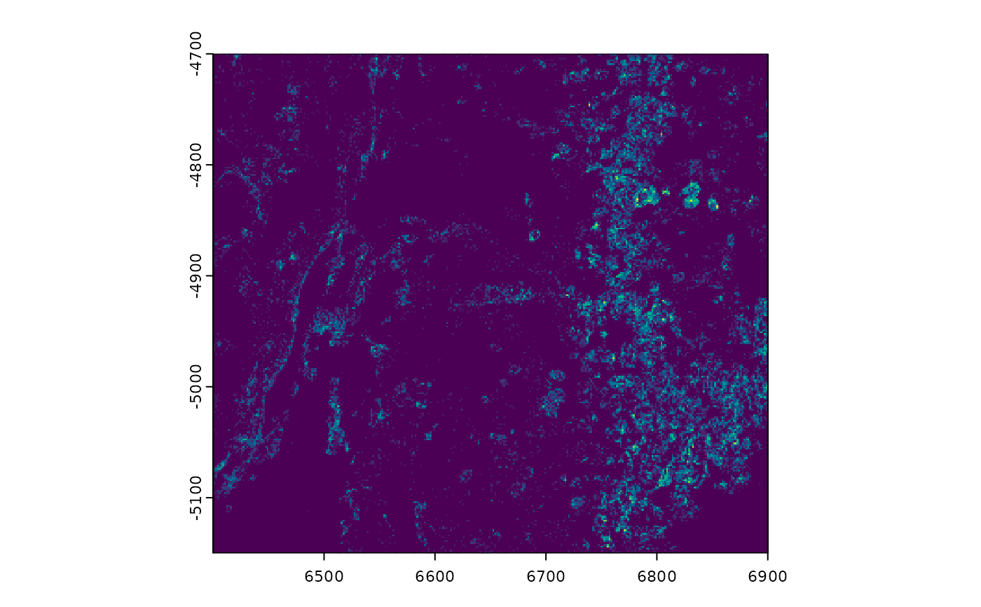
 # plot points density (by count)
plot(gpoints, raster_size = 300)
# plot points density (by count)
plot(gpoints, raster_size = 300)
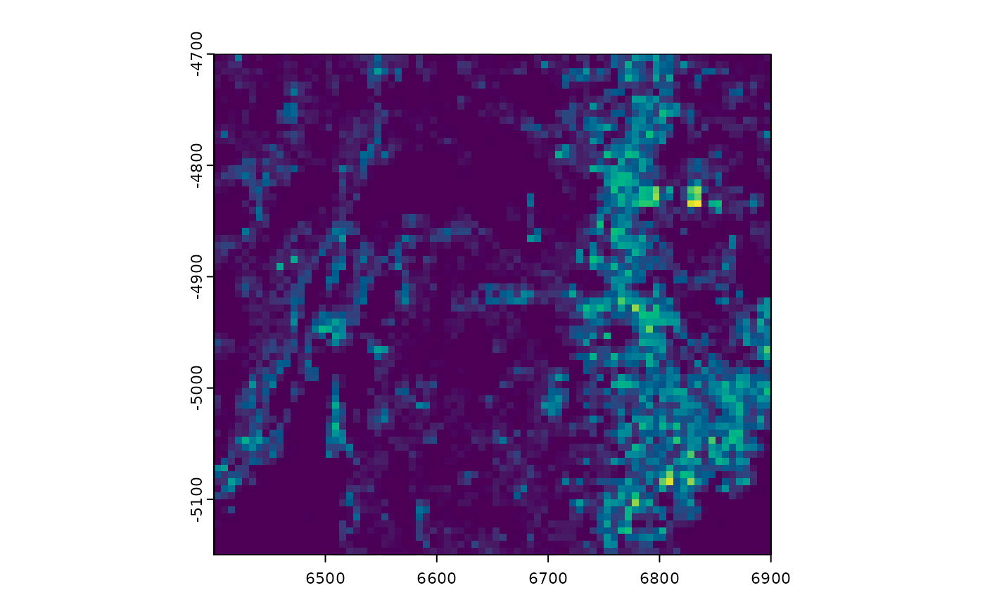
 plot(gpoints, raster_size = 300, sigma = 4)
 # force_size = TRUE to ignore default constraints on too big or too small
# (see details)
plot(gpoints, raster_size = 80, force_size = TRUE)
# force_size = TRUE to ignore default constraints on too big or too small
# (see details)
plot(gpoints, raster_size = 80, force_size = TRUE)
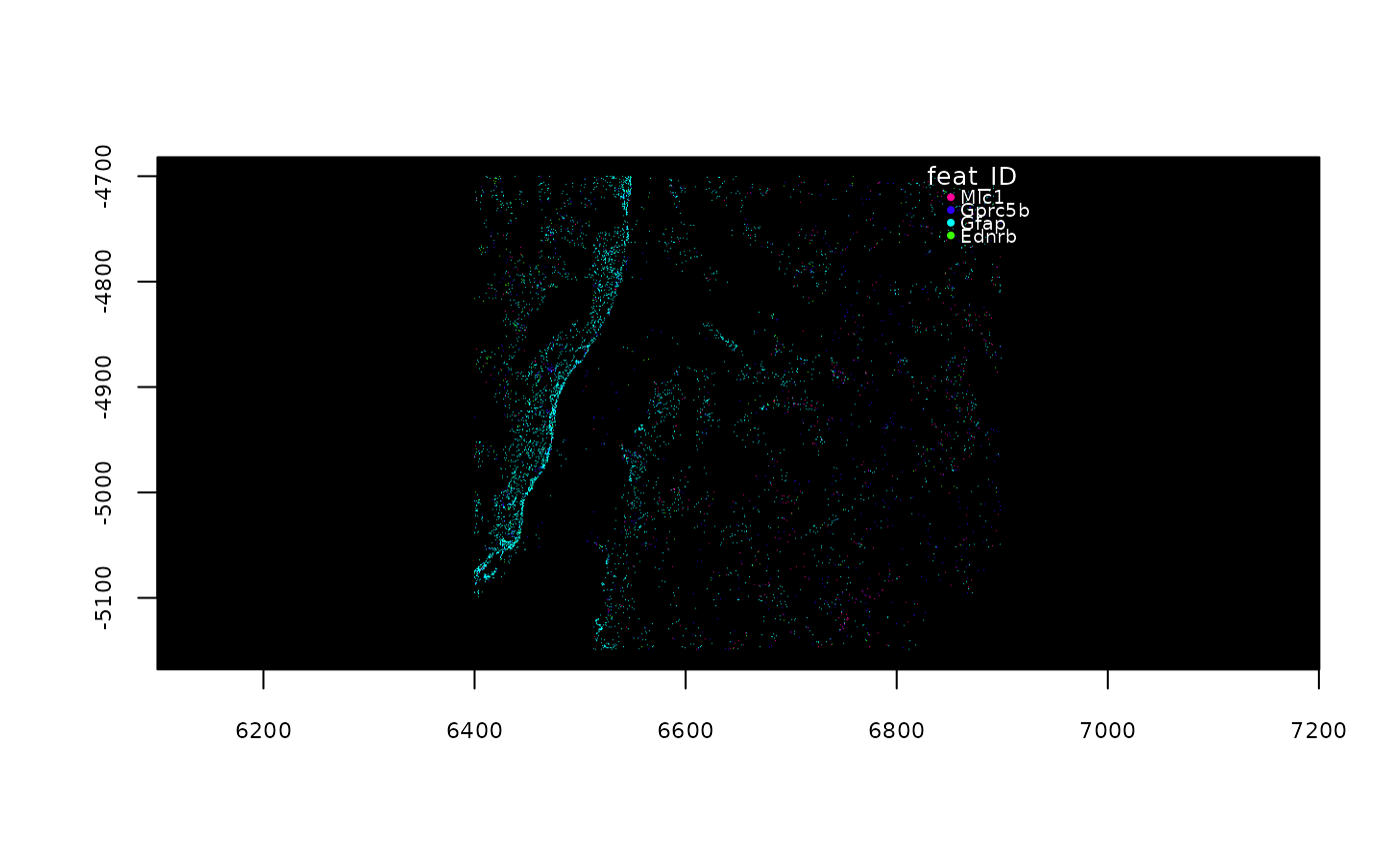 # plot specific feature(s)
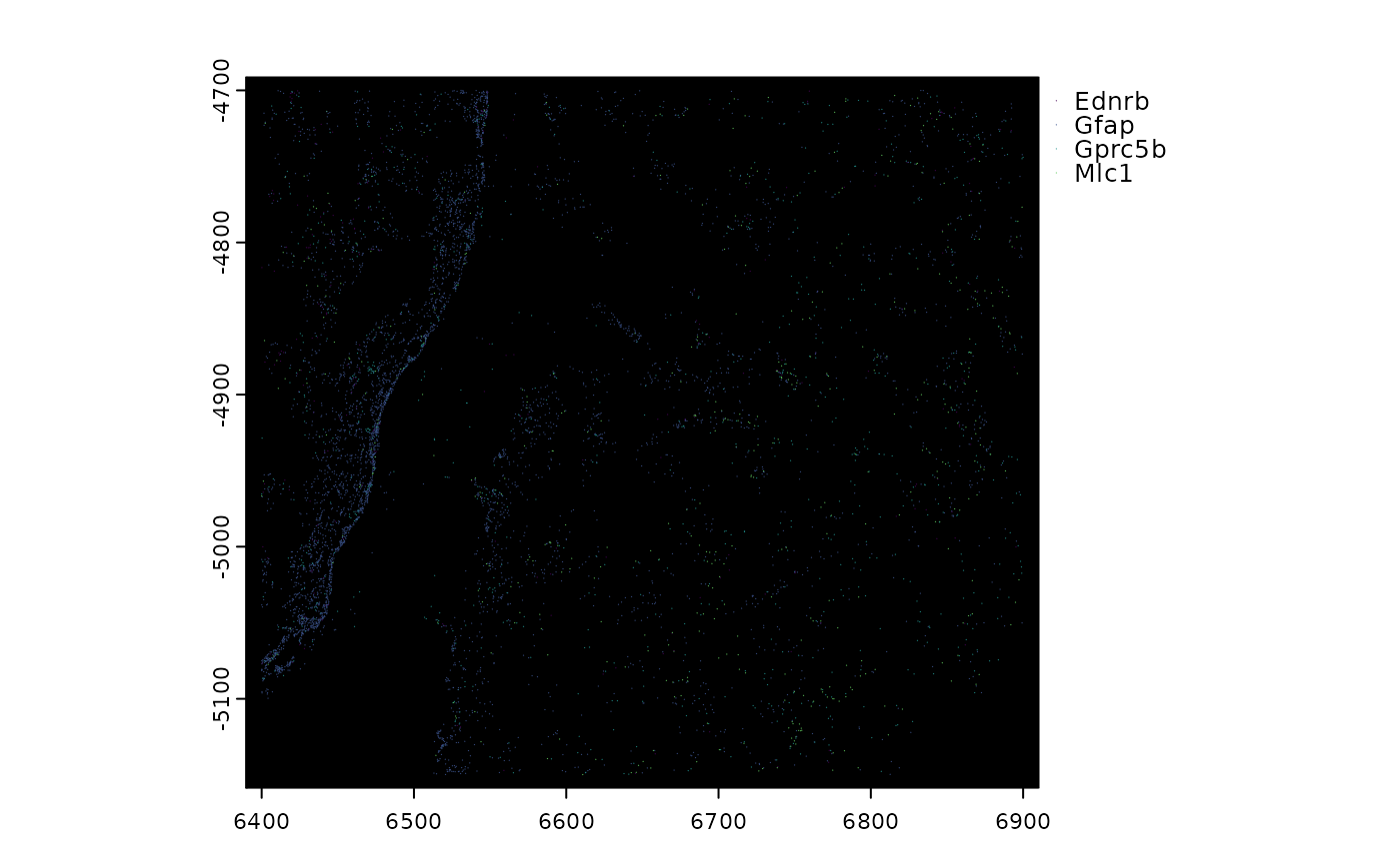
plot(gpoints, feats = featIDs(gpoints)[seq_len(4)])
# plot specific feature(s)
plot(gpoints, feats = featIDs(gpoints)[seq_len(4)])
 # ----- vector plotting ----- #
# non-rasterized plotting (slower, but higher quality)
plot(gpoints, raster = FALSE)
# ----- vector plotting ----- #
# non-rasterized plotting (slower, but higher quality)
plot(gpoints, raster = FALSE)
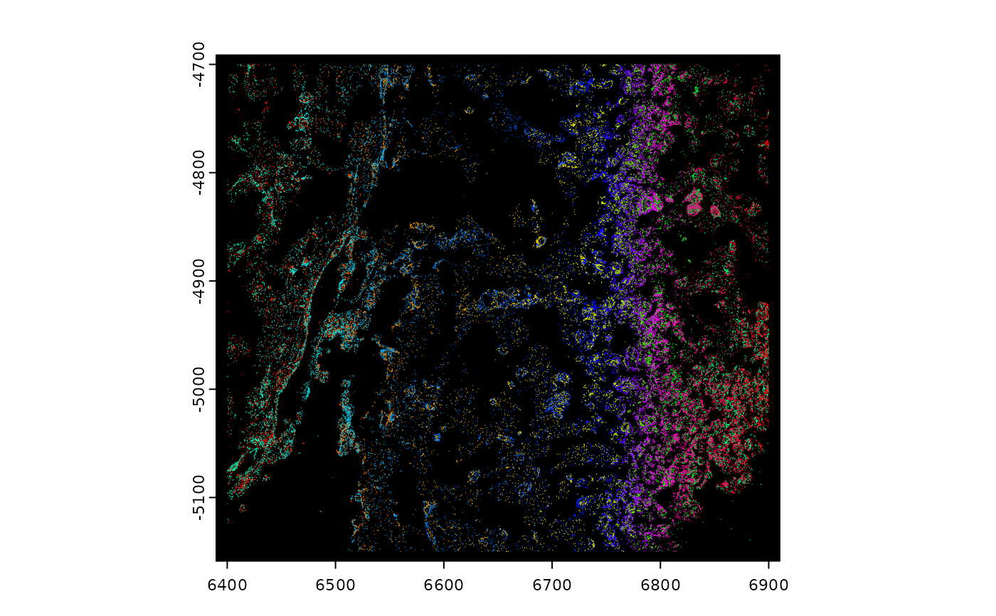 # vector plotting maps colors to transcripts
plot(gpoints, raster = FALSE, col = grDevices::rainbow(nrow(gpoints)))
# vector plotting maps colors to transcripts
plot(gpoints, raster = FALSE, col = grDevices::rainbow(nrow(gpoints)))
 # plot specific feature(s)
plot(gpoints, feats = featIDs(gpoints)[seq_len(4)], raster = FALSE)
# plot specific feature(s)
plot(gpoints, feats = featIDs(gpoints)[seq_len(4)], raster = FALSE)
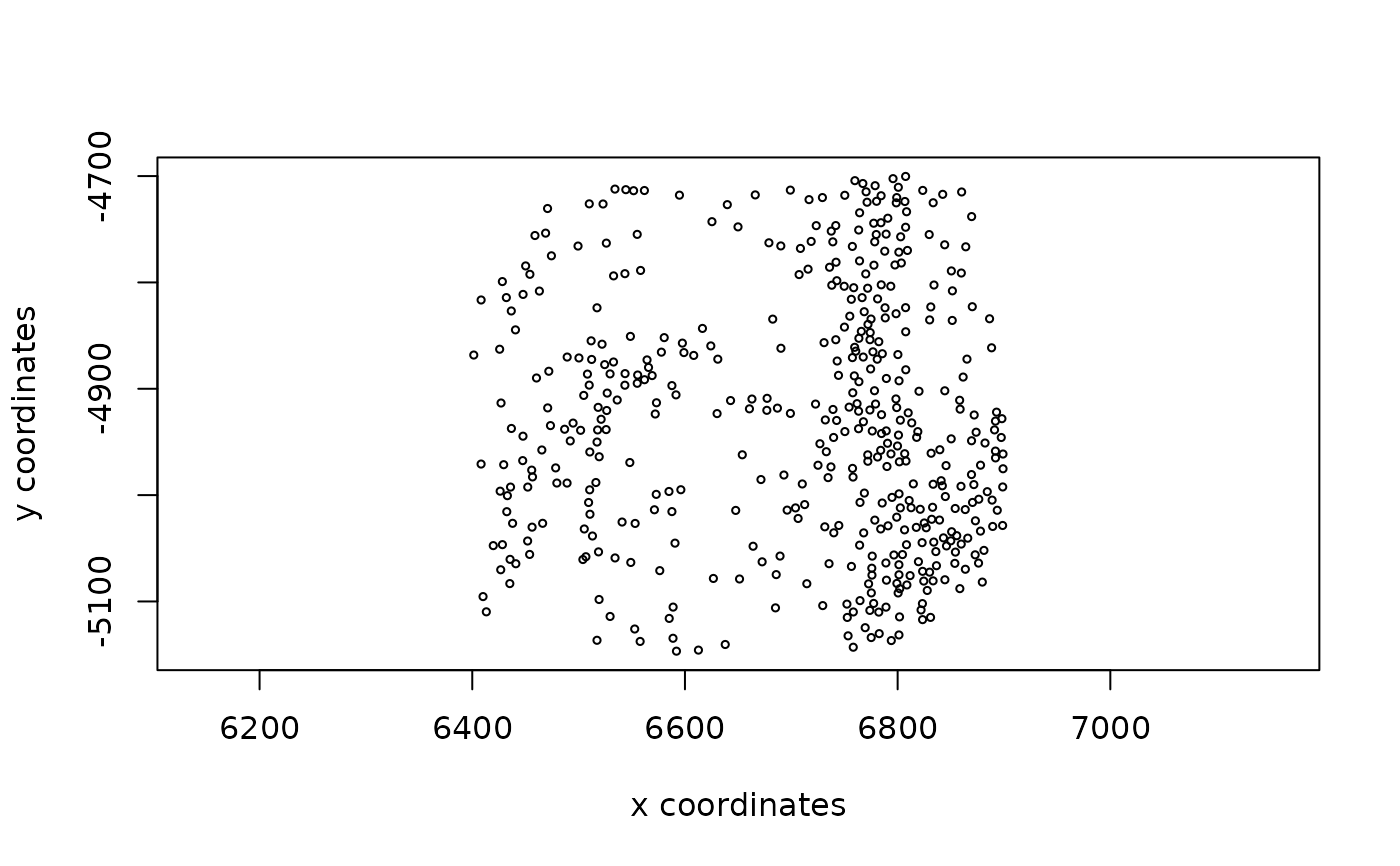 ######### spatLocsObj plotting #########
sl <- GiottoData::loadSubObjectMini("spatLocsObj")
plot(sl)
######### spatLocsObj plotting #########
sl <- GiottoData::loadSubObjectMini("spatLocsObj")
plot(sl)
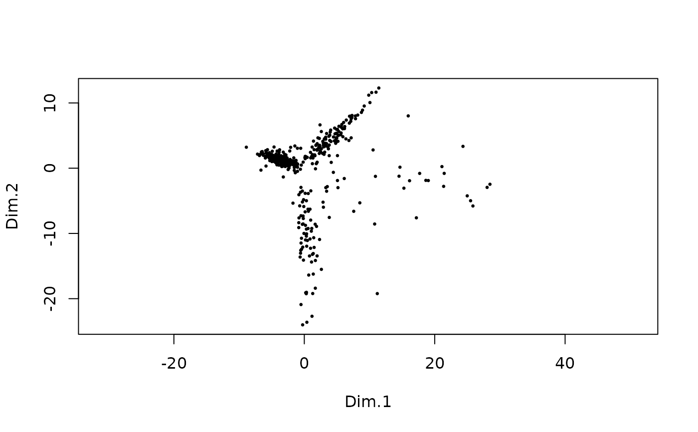 ######### dimObj plotting #########
d <- GiottoData::loadSubObjectMini("dimObj")
plot(d)
######### dimObj plotting #########
d <- GiottoData::loadSubObjectMini("dimObj")
plot(d)
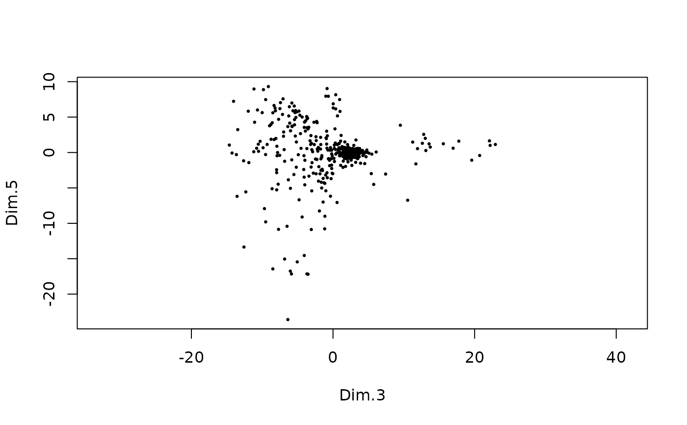 plot(d, dims = c(3, 5))
